Introduction:
The last two blogs focused first on the Recovery and then on the Drive phases of the stroke cycle. Both use actual boat data-logger force measurement derived data from Impulse (F x t) curves, along with rowing tank real-time impulse and handle speed curves as part of the discussions. We will continue to refer to those and similar curves shown below to expand on this discussion.
While the data logger output of impulse, boat velocity, boat acceleration and the subsequent calculation of handle acceleration relative to the moving boat presents the purest rowing force measurement information, it suffers from information overload and from not being able to be viewed in real-time.
Why Use Force Measurement In A Tank:
When used in a rowing tank a force measurement system suffers from the lack of boat acceleration and velocity, however the tank system benefits from being able to observe impulse and handle speed, the same as in the boat. Also, stroke length, gate angle and slip are shown in real time. In addition, each force curve is unaffected by the mass movement of others rowing in the tank. This is an improvement because in the boat the athletes are interconnected, so it is harder to discern who might be creating an anomaly in the curve.
The simulation match between boat and tank is FORCE according to Newton’s 2nd Law: (F = MA), where: M boat x A boat = M of tank water (that impacts the blade) x A of blade. (Note: Nowhere in the simulation equation for force does water speed appear, refuting any reason for a mechanically assisted moving water tank.
Force Measurement In The Boat:
To explain further: Rowing in a moving boat involves the blade of the oar moving through still water. The blade (if correctly buried) only slips relative to the water along a defined path while translating in and out from the boat and generating a component of force that propels the boat forward. The blade follows a curved trajectory first out from the boat and then back tracing a pattern similar in shape to a cursive small letter “e”. A good analogy is to a cam follower being forced to follow the profile of a cam. The water viscosity working against the blade speed reacts similar to a solid surface and resists getting out of the way of the blade, so the blade being fixed to the shaft, which is fixed to the boat at the pin is forced to move relative to the water which flows past the blade, first blade tip to tail and then once past the orthogonal, tail to tip.
In a manner almost directly in contrast, in the rowing tank, the blade is sized small enough so that it can rip through the surrounding water mass to generate its force, following roughly a circular arc. The trick to good tank design is to make the force magnitude represented by the impulse curve (force-curve) and handle speed curve roughly equal to what is experienced in the boat by modulating blade size and oar mechanics.
Once the force simulation is satisfied between the boat and the tank to an acceptable degree than real-time feedback training for rowing can be done in the tank in order to achieve an optimal stroke that is both economical and efficient at near to a racing cadence.
In the tank, the displayed force and handle speed curves become essentially real-time feedback to the athlete that is similar enough to curves downloaded from a boat data logger so that an economic shape of the curve, the area under the curve, and slope of the curve can be mimicked by the rower to achieve synergism. Rowers training in this way will over time quickly converge to near-identical force curve similarity. In short, they will approach a shared optimal rowing technique.
The question then becomes: What does an optimal and efficient technique look like in terms of curve shape, the area under the curve, and slope of the curve? To answer that question, we look for examples of the curves from some of the fastest, most accomplished elite rowers and note what their curves have in common, and how and why they may differ. We then use basic physics mechanics to form a hypothesis that we can use to test less experienced rowers.
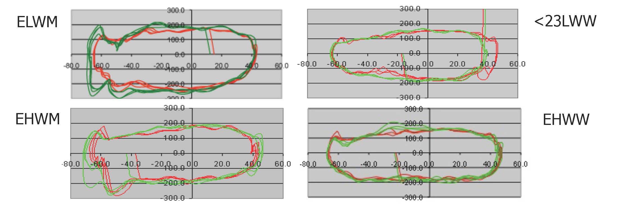
Below are four Curve Sets: (Click To Enlarge the Force Curves With Handle Speed Curve Embedded and See Captions)
Starting from the top left we have: a top US National Team and Olympic lightweight man sculler, a top US multi-National Team and Olympic HW man, multiple Olympic gold medal women, and a US junior lightweight woman sculler (when tested), eventual 2-time under 23 US National team single sculler.
The Catch:
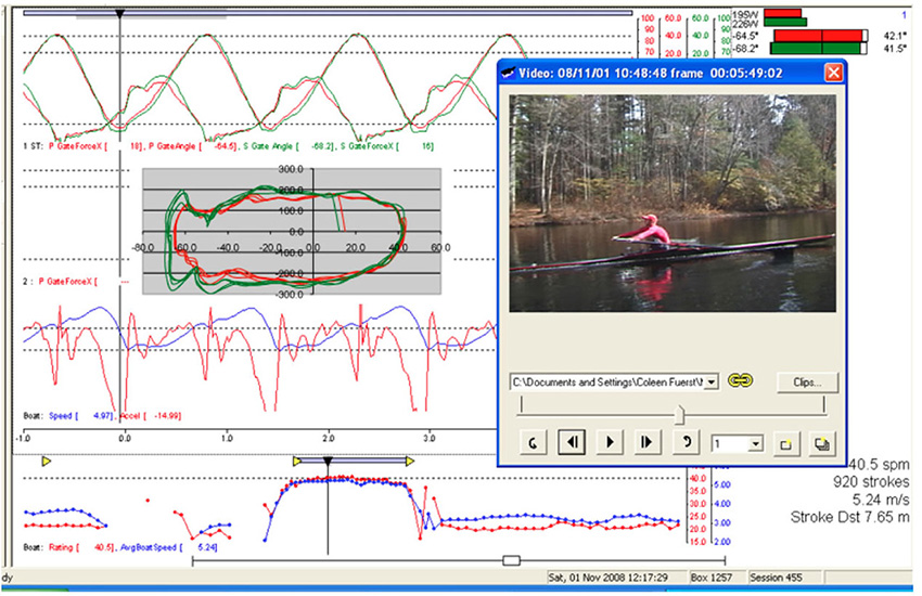
Just below are two sequential curves plus an embedded screen grab video from the LW Male sculler taken just before the catch, and at the true catch. His curves, in general represents a good example of efficient, fast rowing. (Click to Enlarge and See Captions) If you click cycle back and forth you will see in the video how quickly he inserts the blade matching the relative speed of boat to water without any evident body movement other than his hands/arms.
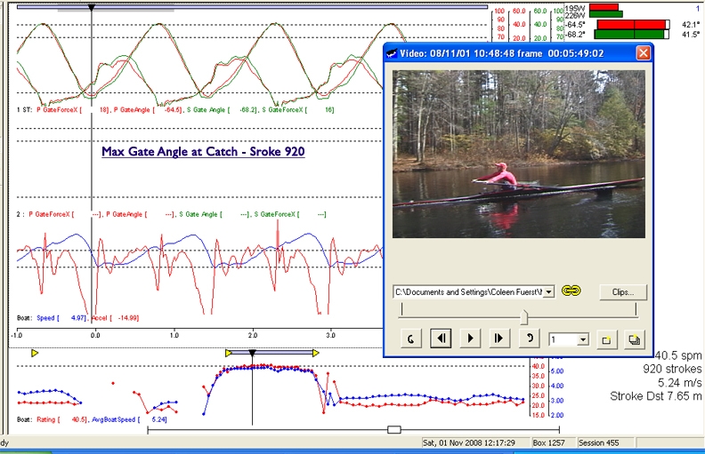
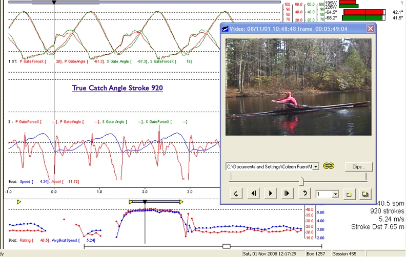
Just below are two sequential curves plus an embedded screen grab video from the LW Male sculler taken just before the catch, and at the true catch. His curves, in general represents a good example of efficient, fast rowing. (Click to Enlarge and See Captions) If you click cycle back and forth you will see in the video how quickly he inserts the blade matching the relative speed of boat to water without any evident body movement other than his hands/arms.
(Click To Enlarge the four Handle Speed Curves and See Captions)
Referring again to the Handle Speed Curves of the four examples of quite accomplished scullers. You will see the same characteristic curve at the catch with all of them where the handle speed is constrained by boat speed. The point that this makes is the futility and inefficiency of driving too hard with the legs initially. You must limit force until the boat progresses enough to have a favorable mechanical advantage with the leg angle. About 75% of maximum pressure will be enough until the legs get to a biomechanically strong position to be able to drive down hard.
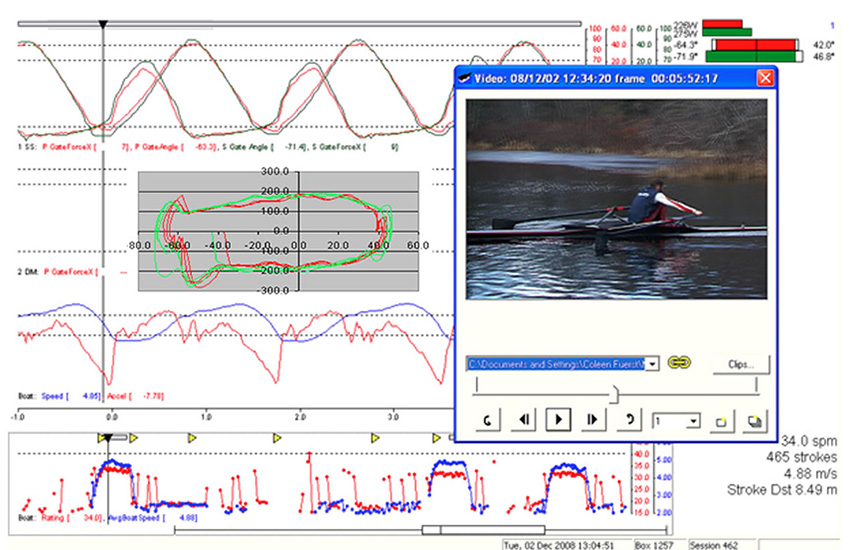
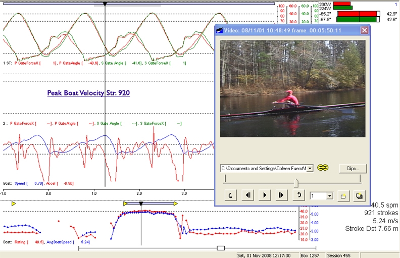
The Drive:
(Click to Enlarge and See Captions)
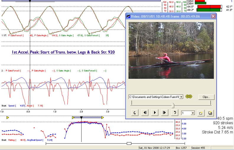
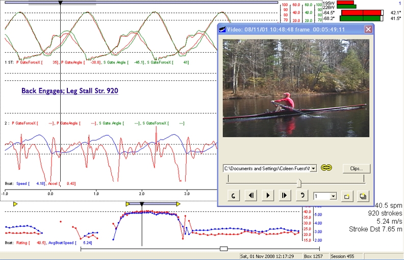
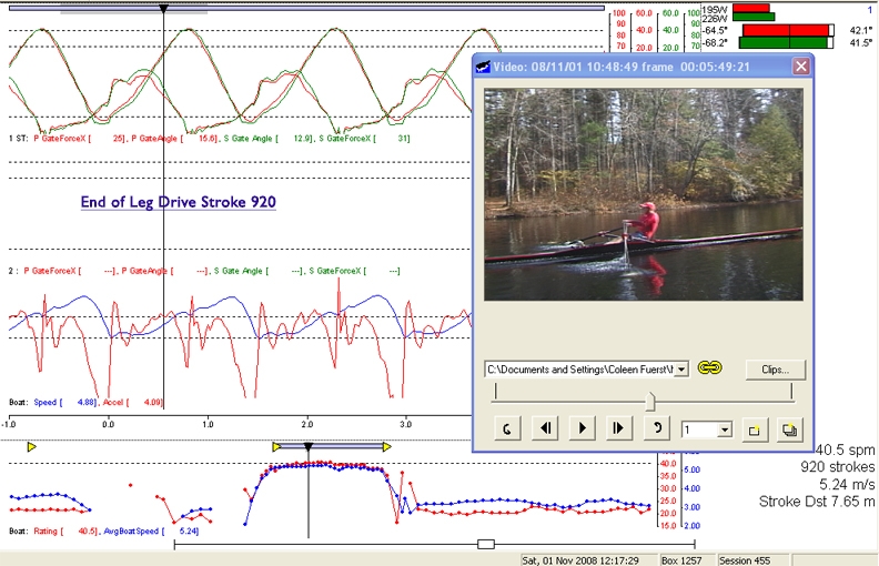
Notice that as the drive progresses the boat velocity stays at its minimum until well past the orthogonal position (when the oar is perpendicular to the boat). From there until the end of the stroke the rowers mass (which is about 6 times the boat mass), is trying to move the boat in the wrong direction – toward the start rather than the finish line). This mass resistance becomes exponentially less as the drive progresses, allowing the boat to accelerate and the velocity to increase due to oar handle acceleration. (i.e., shown by an increasing slope of the blue velocity line). At the same time, the handle speed curve has a noticeable upward slope from 100 radians to 200 radians. While the blade is in the water the steeper the slope of the handle speed curve the faster the boat. Boat velocity and handle speed are of course directly related.
When rowing in the tank where there is no boat velocity. Tank handle acceleration is shown by the upward slope of the handle speed curve on the drive (i.e., top of the curve from left to right). This technique must be achieved without “washing out”.
The best shape of the impulse curve is a full curve slightly rounded on the top. Trapezoidal is even better, even our young sculler’s curve shows this, taking into account her inexperience at the time with much less power and a slower catch. What you don’t want is a narrow high peak curve.
In general, the larger the area under the impulse curve, the better. (i.e., with the area being the integral of the curve).
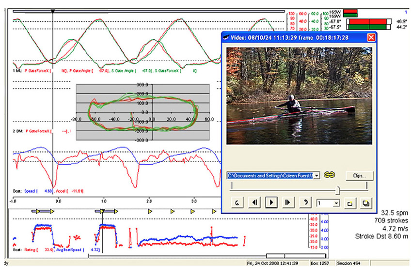
The Recovery:
The 2nd part of the stroke – the recovery, can best be thought of as the other side of the equal sign in Newton’s 2nd law. It is Mass times Acceleration M x A, whereas the Force part of F = MA can be considered to be the drive and the Mass x Acceleration the recovery. You may ask what mass are we referring to? It is primarily the rower’s mass since it is approximately 6 times that of the boat. During the drive phase of the stroke, we use our kinetic energy (i.e., 1/2 mass times velocity squared). This energy is now available as the potential energy of position (with no gravity to help us, except for the slight incline of the slide). The effect of this available energy is graphically shown by the large boat velocity increase during the recovery to maximum boat speed just before the catch solely due to the mass movement of the rower from finish to catch. This increase in boat velocity on the recovery is at least equal to, or more than that seen generated from Catch to Finish during the drive. This is despite boat frictional resistance increasing as the square of the speed.
Rewriting Newton’s 2nd law results in the Impulse/Momentum equation F x t = M x V. This should be familiar since Force and Time are the x, y coordinates for the Impulse (force) curves and F x t is the definition of impulse. Since Impulse equals Momentum we can define the rowing stroke (cycle) as Drive velocity is the result of Impulse and the recovery velocity the result of momentum.
Recovery in the tank: We don’t have boat velocity or acceleration curves in the rowing tank, and there is no useful driving force on the recovery in the tank from momentum because of the literally astronomical reversal in mass ratios from our predominant 6 to 1 when considering our mass to the boats mass which is supported by an almost frictionless surface of the water, as compared to the mass of the earth which we are affixed to!
Recovery on the water: However, the handle speed curve clearly shows that the Recovery (bottom horizontal) is almost a direct mirror of the Drive (top horizontal). It shows what our mass is doing because it is connected to the handle. Two of our model male scullers show a very nice mirroring of the handle speed on the recovery. When done correctly the complete handle speed curve shape resembles that of a snack food “little fish”.
What the recovery part of the curve shows is a measured speed after the hands come away with the upper body swinging forward and the rowers mass moving toward the Catch (left the vertical side of the curve) at a velocity about equal to that of the drive, or about -200 radians at racing rates. The rowers mass then speeds up in conjunction with the square up just before the catch in an effort to continue the momentum and make de-acceleration of mass as short as possible.(Click to Enlarge and See Captions)
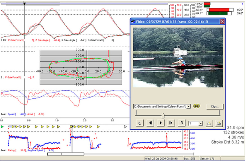
Instantaneous Tank Display:
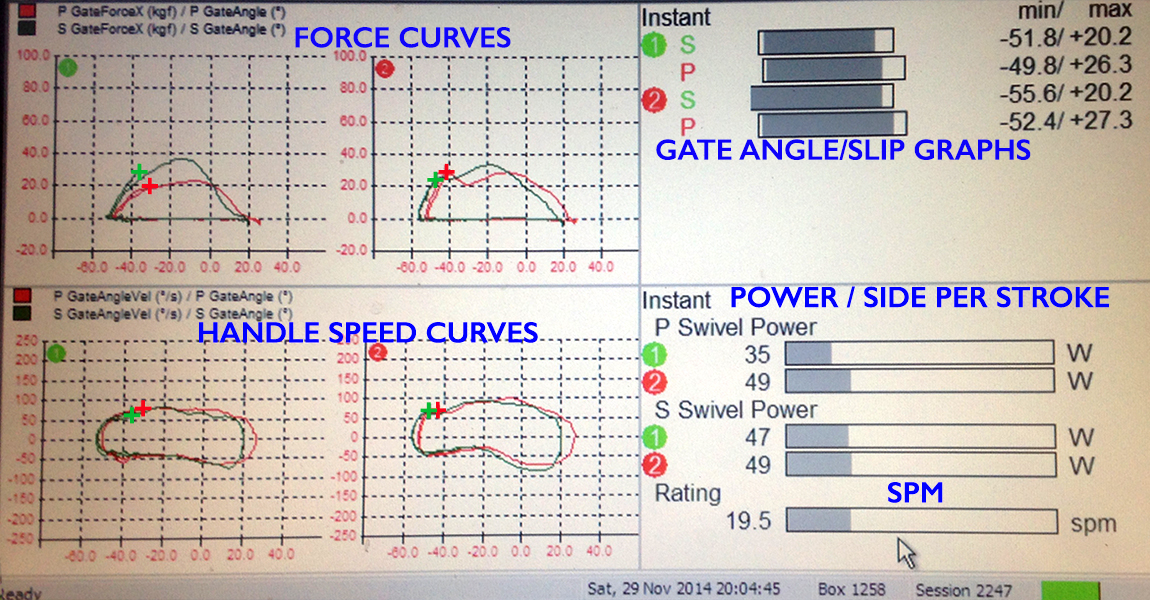
Below are data curves from a display in an indoor sculling tank equipped with force measurement instrumentation. Shown are instantaneous Force Curves (Impulse Curves) and Handle Speed Curves with a red “+” indicating the position of the port hand and a green “+” for starboard hand, which also indicates the relative positioning of the hands on both sets of curves. Note the bar graphs on the right side are refreshed once per stroke. The curves are from two 16-year-old scullers so we try not to be too judgmental. The more accomplished sculler is on the right (stroke) side. The less accomplished with regard to technique is on the left (bow).
Reading the display going clockwise: Force curves are in the upper quadrant for both rowers with a red dot indicating port and the green dot starboard. The next quadrant shows handle speed represented as a bar graph with the length of the bar representing stroke length and the relative starting point of each bar indicating the furthest catch angle for each side for each rower. Numerical catch angles are to the right of each bar. There is a threshold value of ten newtons that has to be exceeded before the bar is shaded and that visually represents the true catch. The length of shading represents total effective stroke length until the 10-newton threshold is crossed again. The goal here is to have no white showing at the start of the bar, indicating a quick catch. It is almost impossible to eliminate all the white at the end of the bar due to momentum. However, an excessive length of “white” indicates premature disengagement from the water (i.e., washing-out or pulling down into one’s lap) indicating less efficiency.
The 3rd quadrant shows power per side for each sculler in watts and stroke rate. This is not absolute power but relative power because the mechanics of the tank are so much different from the boat that it is beyond the calibration range of the software.
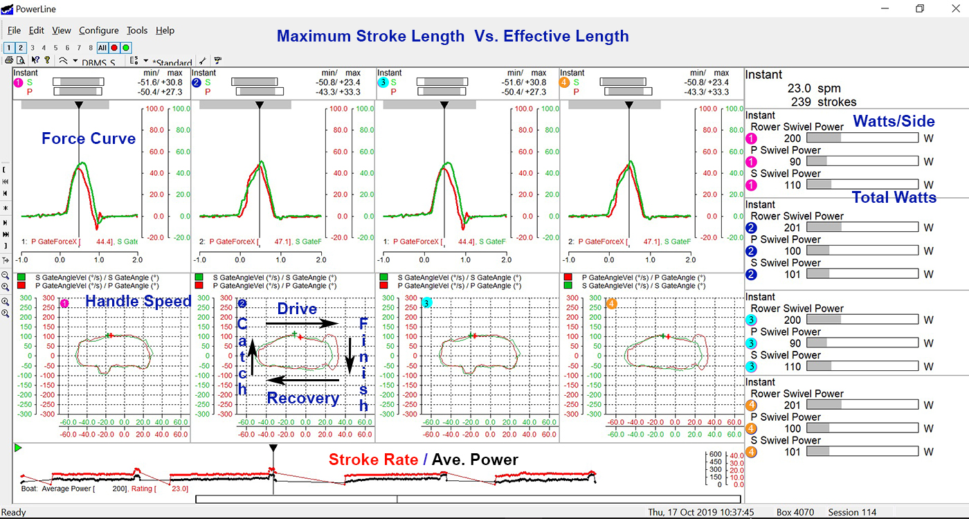
The last quadrant shows the handle speed for each sculler. The shape and slope are similar to that seen in the boat, with the exception of immediately after the catch is more continuous mainly because the blade is being pulled through the water rather than being supported by the water and forced to match boat speed, as in the boat. The shape of the handle speed curve ends up looking like a “peanut”, curved downward at both ends with top and bottom mirroring one another. The second report shows an output report showing data for four people
(Click To Enlarge of Two Different Sample FM Data Screens)
The above video shows the same two young scullers using the tank. You can hear me coaching them by questioning them: “When you accelerate your hands at the end of the stroke, what does that do to the shape of the (handle speed) curve?”. In this way, they learn by doing, assisted by real-time feedback. This is a much quicker, and more long-lasting coaching method, that works so much better than hoping that they will interpret your words correctly.
From experience, we have learned that if the rower is self-coaching in the tank, he or she can only effectively look at one quadrant at a time. By playing the video over-and-over you should see most of the following takeaways: The bow person (left side) has trouble with the side-to-side synergism as compared to the stroke person (right side). The slope of the curve at the Catch is different between the bow and the stroke, and this is also reflected in the slip at the catch shown by the bar chart. What you don’t see or know is that the person in stroke-seat has primarily sculled, whereas the bow person has primarily rowed sweep. The bow person is quite a bit taller while being short in the water on each end of the stroke. You can see that there is less handle speed acceleration during the stroke with the bow person than the stroke. There is a different hand speed away from the release of the recovery by the two athletes, which does not help synergism. The bow person is a bit excessive with hand speed out of the bow.
Problems like these can be easily seen and identified by the rowers in real-time as well as by the coach. From our experience, identical problems occur on the water and in the tank. Once pointed out, the problems can usually be quickly fixed.
During the practice, a video can be made of the output data along with a video of what the problems look like from the stern or side-view and sent via cell phone immediately to the athlete. This a very powerful tool. When environmental conditions of wind and weather, or school constraints impact training time, then real-time tank sessions are a much better use of coaching time then on-the-water sessions.
In boat-handle acceleration is shown by an increasing slope of the blue velocity line. Generally, the handle speed curve has a noticeable upward slope from 100 to 200. While the blade is in the water the steeper the slope of the handle speed curve the faster the boat. Boat velocity and handle speed being directly related.
When rowing in the tank where there is no boat velocity the tank handle acceleration is shown by the upward slope of the handle speed curve on the drive (i.e., top of the curve from left to right). This technique must be achieved without “washing out”.
In the tank, the best shape of the impulse curve is a full curve slightly rounded on the top. Trapezoidal is even better, even our young sculler’s curve shows this, taking into account her inexperience at the time with much less power and a slower catch. What you don’t want is a narrow high peak curve.
See following video taken last Fall;
In general, the larger the area under the impulse curve, the better. (i.e., with the area being the integral of the curve). The above video was done at Steady State. The following was done to maximize synergism with the Force Curves peaks.
By: Jim Dreher and Coleen Fuerst
Leave a Reply