Explanation:
A little explanation is in order: This first page is meant to simply and briefly explain the theory and mechanics behind the analyses of the rowing stroke. The following three pages are executive summaries for rowers and coaches again respecting short tension spans in the interest of brevity. The meat of this tome follows with occasional references to the durhamboat.com website for video and curve info.
Each rowers force measurement curve and handle speed curve will have it’s own unique shape and characteristics which are capable of being identified as a signal. Other “signals” can be had from basic physics properties such as velocity, acceleration, distance and time or combinations such as impulse and momentum. Even the displacement of the centroid of the force curve area can serve as a signal when compared to a template of an “ideal” template curve.
Once a signal is chosen then a sensor (transducer) has to be chosen to detect the signal and convert (transduce) it in the form of digital electrical data. Typical transducers are a strain gage to measure oar deflection, a force transducer to measure the resolved forward force on the pin, an accelerometer to measure the momentum of the rower on the recovery part of the stroke, or an encoder or solid state gyro meter to measure angular velocity of the oar, or what we refer to as ”handle speed”.
Software code (algorithms) must then be written to detect, classify and interpret the signal To report back to the rower (in real time.) so that the rower can correct his/her movement and make it more efficient. The above description should sound familiar to any rower who has been coached. What is described above is best thought of as an Augmented Reality Rowing Coach!
The signal quantifies the kinetic energy of the rower. For example: If we use a graphical description of force x time we have plotted Impulse, which equals Momentum (mass x velocity). The area under the curve is the total energy expended during the drive.
Executive Summary:
What do the curves tell us?
Summary for the rower: There are five basic principles shown by the curves that could have an immediate effect on making your rowing technique more optimum, and result in you being able to row faster with less effort:
Focus on always having a quick, deep catch;
Have the patience to not push or pull too hard right after the catch (immediately put on no more than 75% maximum pressure;
then let the boat speed put you in a mechanically favorable position, and only then apply maximum pressure with the focus being on handle speed all the way to the end of the drive phase of the stroke cycle;
Have a measured (even) speed of your body mass on the recovery that “mirrors” the drive speed;
Delay the square up until the last possible moment (flip-catch) accompanied by a slight acceleration of the body mass to preserve momentum.
The first three principles are the results of rowing physics described by the graphs that govern the drive portion of the stroke cycle and are based on the optimization of Impulse (F x t). The last two principles (also part of the 2nd principle) are based on optimization of Momentum (M x v), which governs the recovery.
To drill down and simplify further, there are three things to focus on during drive and recovery:
Drive: A quick, vertical catch, then 75% max pressure immediately, followed by full pressure handle acceleration until the release.
Recovery: Mirror the drive velocity, with hands and upper body quick out of bow, then the constant velocity of body mass until near the end of the slide, followed by a slight acceleration of mass coincident with a “flip” catch.
FAQ for the Coach:
What is the importance of “mirroring” when describing the handle speed curve?
There has to be symmetry of Impulse and Momentum. The handle speed curve is a 360-degree curve, so the zero datum coordinate line bisects it horizontally with the drive (impulse) being + and above the datum, and with the recovery (momentum) being – and below the zero coordinate datum. The optimum handle velocity profile appears as a “mirror” image of the recovery as compared to the drive. For example: If the drive oar angular velocity (handle speed) is + 200 radians at the orthogonal position than at the same orthogonal position on the recovery it will be about -200 radians.
How do you ”force curve match” to synchronize a crew using rowing physics?
In the boat, you start with all rowers having an identical catch angle by having the crew come to their furthest extension possible, and then adjust and match all to the stroke position’s catch angle by moving foot stretchers, etc. You will now have at least a common starting point with all experiencing the same lift vector angle at the catch position regardless of each rower’s relative force potential. From that identical starting position, each will have a slightly different curve with a different maximum peak force. The trick will be to synchronize the different peak forces of each rower, so they all achieve maximum force at close to the same time. This is called “force curve matching.” Of the two physics properties that you are attempting to match – force and time, only time is possible to match. Maximum force is specific to each individual, but timing is everything! Ideally, the peak force of each curve measured on the vertical axis and all eight curves should nest like 8 Russian dolls, each one inside the other. Time on the horizontal axis will mark the centerline of the nest.
Force times time is the definition of Impulse, so the area under the curve is the Impulse. Impulse in rowing is the drive portion of the stroke cycle when the oar “drives” the boat velocity from it’s minimum to only its average velocity at the end of the drive portion of the stroke cycle.
It is easy to deduce that a large, full area under the impulse curve will be more powerful and efficient than a high but narrow triangular shape over the same time period, with the result being a higher average boat velocity going into the recovery portion of the stroke cycle.
An economic shape of the curve will have a full area under the curve. To the extent possible, the slope of the stroke curve, just after the catch should be mimicked by others in the boat to achieve better synergism. Rowers training in this way will over time quickly converge on near identical force curve similarity. In short, they will approach a shared optimal rowing technique.
There must be an optimal curve, but as a practical matter, a crew may approach the optimum, but it is unlikely that a crew would ever find it due to training time limitations. What an optimal curve representing efficient technique looks like in terms of shape, the area under the curve and slope of the curve is academic. It is best to select your best rower as the stroke and then train the other seven to match his force application in timing. Force amplitude will take care of itself as a result of training.
As the drive progresses, the boat velocity stays at its minimum until well past the orthogonal position (when the oar is perpendicular to the boat). Training involves developing the skill level of following the strokes force curve, matching him in the timing of his peak force, and in oar angular velocity right to the end of the drive. The faster sweep boats tend to imprint a “sequential” style (i.e., first legs, than back and arms) and scullers, especially a small boat sculler tend to row in more of a “simultaneous” manner. This is meaningless in practical application because each rower will use his individual body parts – legs, back and arms in slightly different ways and sequences. All that matters is synergism of force application relative to time. Force amplitude to a certain degree is desirable, but timing the force application is the most important variable in a crew boat.
What is the next step to achieve synergism?
Once the catch angles and force curve peaks match (be patient, it will likely take time). Then we work on rounding out the curve profile. This is nothing more than increasing the area under the curve while at the same time preserving the relative “nesting” of each individual curve within the others. This can only be done by increasing handle speed, accompanied by force within what each rower is capable of, while at the same time not changing the peak force location. This can be done at moderate training stroke ratings with the extra effort given to increasing handle speed a little closer to the catch and especially by getting faster close to the finish. Usually, just a mental note to increase handle speed will do the trick and you will round out the first part of the curve and turn the finish profile concave to convex.
What other curves could be used for real-time feedback of synergism?
I propose that a curve, bar chart or perhaps some other chartable algorithm be created that shows each rower’s Centroid of the area under the force curve.
The centroid of the impulse curve is unique for each individual as it defines the point in time during the drive portion of the stroke cycle that the total of the rower’s energy is centered independent of maximum force and shape of the curve. Real-time feedback of each rower’s centroid as compared to the strokes centroid would be the ultimate measure of synergism. Perhaps a graph consisting of a vertical series of lines where the goal would be to superimpose each rower’s line over the strokes until only one thin line shows.
Introduction:
A less formal title for this dissertation should have been “Learn a little physics and a lot about optimizing rowing technique.” The two are conjoined because rowing is such a mechanical, technical and equipment based sport.
Rowing as a sport started with the goal to get from point A to point B faster than your competition, and it has been around for a long time as a form of transportation, commerce, warfare, and sport.
Early on strength, endurance, technique, and equipment were recognized as the keys to winning rowing races. While the first two: Strength and endurance are givens, rowing technique, and the latest equipment are the wild cards that determine the winners from the losers. This was just as true when rowing boats were used as war machines, such as the Greek Triremes 2500 years ago in the Peloponnesian wars, as it is today with the lightweight all carbon racing machine of the modern Olympics. The common thread being the word: Machine.
With an apology to cycling; Rowing is the only total body involved sport where the rower is the engine in a kinematic machine. Kinematics is a Physics Mechanics term describing how machines work, i.e., how the geometry of the various gears and levers rotate relative to each other, but without regard to the forces that make them move. To show forces we use force vectors of relative magnitude due to their length and direction in a kinematic analysis.
The rowing stroke is all about energy transfer. During the drive portion of the stroke cycle, the rowing mechanism works when the rower applies a force thereby increasing the potential energy of the rower’s mass. Then during the recovery portion of the stroke cycle, the rower converts this potential “energy-of-position” to kinetic energy as the rower’s mass moves back to the starting point, the catch.
An actual energy balance analysis would not only be near impossible to do and would serve no practical point. However, the above rather simplistic description of the rowing stroke is meant to show that energy is continuously being expended, stored and used throughout the complete stroke cycle to maintain and increase the boat velocity, not just during the drive.
The goal of kinematic analysis of the stroke cycle should be to identify how to efficiently use the limited energy resource that is available to the rower.
An important observation is that throughout the stroke cycle until just before the next catch the velocity of the boat continues to increase, reaching a maximum just before the next catch. This cycle continues to work to increase boat velocity because even when the oars are out of the water the rower’s mass creates momentum by freely moving relative to the much lighter boats mass.
A kinematic analysis of the rowing motion would describe a complex mechanism that follows the basic physical principles of Physics Mechanics.
About 350 years ago Newton wrote his Principia in which he stated the 2nd of his three laws of Physics: F = MA (force is equal to the mass of an object times its acceleration).
There are four basic properties in Physics: Force, Mass, Distance, and Time. Others such as Velocity, Acceleration, Impulse, and Momentum are derivatives of the basic four and all are used to understand what an optimum rowing motion should look like when graphically displayed. A graphical display of Force times Time is, in essence, a kinematical analysis.
Studying a graphical display of force, ideally, in real time, both rowers and non-rowers alike can derive an optimum stroke profile, and experience and learn physics mechanics by doing it heuristically.
The indoor rowing tank is in some ways better than the boat to display and observe a stroke profile because it becomes a virtual physics lab, isolated from the environment and interference from other rowers.
Force Measurement In The Boat vs. Rowing Tank:
To study the rowing motion with the goal being to achieve an optimum rowing technique we must use physics.
Newton was a mathematician who found it necessary to invent Calculus to explain Physics, but numbers by themselves poorly explain the complexities of a machine. For that, we need a kinematic analysis using points and vectors showing both the direction and the magnitude of the forces. But this becomes hopelessly complex, especially with the human body and all of its moving bits and pieces immersed in this mechanism.
This complexity can be eliminated with a real-time graphical display that shows the net result of all the kinematic interactions of the body/oar/boat in the form of a graphical output in terms of Physics properties: Force, Time, Mass, and Distance, plus their derivatives of Velocity, Acceleration, Impulse and Momentum. This is the digital display commonly referred to as a Force Measurement System, or FM System.
The FM System display can be mounted in the boat or rowing tank at each station, or it could be a large screen TV for all to see in the tank room. An in-the-boat display is challenged by the distractions of the environment and the interactions of other rowers. Also, the display must be large enough and mounted high enough so that the rower is not forced to look down at it.
The most common display shows what is called a “force curve”. It is “force” on the vertical axis and “time” on the horizontal axis of the coordinates.
Force times time is the definition of Impulse, so the area under the curve is the Impulse. Impulse in rowing is the drive portion of the stroke cycle when the oar “drives” the boat velocity from it’s minimum to the average velocity of the stroke cycle.
Your mind can easily deduce that a large, rectangular area under the impulse curve will be more powerful and efficient than a high but narrow triangular shape over the same time period, and result in a higher average boat velocity. You can easily make adjustments “on-the-fly” via your visual system to match your curve to any “template” optimum curve in real time.
Momentum in rowing is the recovery portion of the stroke cycle. The 2nd part of the stroke – the recovery, can best be thought of as the other side of the equal sign in Newton’s 2nd law. It is during the recovery that the potential energy (energy of position) is converted to kinetic energy (energy of motion) resulting in the maximum boat velocity being achieved just before the next catch.
The Force part of F = MA can be considered to be the drive and the Mass x Acceleration the recovery. You may ask what we are referring to regarding mass? It is primarily the rower’s mass since it is approximately 6 times that of the boat.
As mentioned before: During the drive phase of the stroke, we generate potential energy. During the recovery, this energy is now available as potential energy of position (with no gravity to help us, except the slight incline of the slide). During the recovery, we convert this energy into kinetic energy. (i.e., 1/2 mass times velocity squared). The effect of this available energy is graphically shown by the large boat velocity increase during the recovery to the maximum boat velocity seen during the entire stroke cycle, which occurs just before the catch, solely due to the mass movement of the rower from finish to catch. This increase in boat velocity on the recovery is at least equal to, or more than that seen generated from Catch to Finish during the drive. This is despite boat frictional resistance increasing as the square of the speed. This shows that there is great potential for boat speed improvement by controlling momentum (mass x velocity) on the recovery. This observation is not new, and was expressed by the famous Australian/British coach Steve Fairbairn over 100 years ago when he said: “Find out how to move your weight, and you will solve the problem of how to move the boat.”
Rewriting Newton’s 2nd law by multiplying each side by “time” results in the Impulse/Momentum equation F x t = M x V. This should be instantly recognized since Force and Time are the x, y coordinates for the Impulse (force) curves and F x t is the definition of impulse. Since Impulse equals Momentum, we can define the rowing stroke (cycle) as The Drive velocity is the result of Impulse and Recovery velocity the result of momentum.
Below is a discussion on how the basic rowing physics principles can be applied by using force measurement as a feedback device to self-coach with the objective to achieve the optimum, most efficient stroke based on the physics of rowing.
Feedback:
Coaching is feedback to the rower by way of an interpreter – the coach, and something always gets lost in translation. By using a Force Measurement display that intermediate step is eliminated. What you see is what you get, and you can make a change instantaneously! But first, we must know what the optimum, most efficient rowing stroke model looks like, and then apply the rowing physics basics to replicate the optimum stroke.
Rowing in a moving boat involves the blade of the oar moving through still water. The blade (if correctly buried) only slips relative to the water along a defined path while translating in and out from the boat and generating a component of force that propels the boat forward. The blade follows a curved trajectory first out from the boat and then back tracing a pattern similar in shape to a cursive small letter “e.” A good analogy is a “cam follower” being forced to follow the profile of a cam. The water viscosity working against the angular velocity of the blade reacts as if it was a solid surface and resists getting out of the way, so the blade is fixed to the shaft, which in turn is fixed to the boat at the pin. The blade attached to oar-shaft and pin is forced to move relative to the water first from tip to tail and then once past the orthogonal, tail to tip.
In a manner almost directly, in contrast, the rowing tank blade is sized small enough so that it can rip through the surrounding water mass to generate its force following roughly a circular arc. The trick to good tank design is to make the force magnitude represented by the impulse curve (force-curve) and handle speed curve roughly equal to what is experienced in the boat by modulating blade size and oar mechanics.
The simulation match between boat and tank is Force according to Newton’s 2nd Law: (F = MA), where: M boat x A boat = M tank water (impacting blade) x A blade. (Note: That nowhere in the simulation equation for force does water speed appear, because the water is treated as a resisting mass that the rower pushes against in the boat or treated as pushing through the water in the case of the tank, refuting any reason for a mechanically assisted moving water tank.
Once the force simulation is satisfied between the boat and the tank to an acceptable degree than real-time feedback training for rowing can be done in the tank to achieve an optimal stroke that is both economical and efficient at near to racing cadence.
The displayed force and handle speed curves become essentially real-time feedback to the athlete that is similar enough to curves downloaded from a boat data logger so that an economic shape of the curve, the area under the curve, and slope of the curve can be mimicked by all to achieve synergism. Rowers training in this way will over time quickly converge on near identical force curve similarity. In short, they will approach a shared optimal rowing technique.
The question then becomes: What does an optimal and efficient technique look like in terms of shape, the area under the curve, and slope of the curve? To answer that question we look for examples of the curves from some of the fastest, most accomplished elite rowers. Then note just what their curves may have in common.
To define an optimum technique, we must refer to the basic rowing physics principles that have been outlined above along with actual FM data from both the boat and the tank to prove to ourselves what in theory might make a boat go fast and at the same time use the least energy. We then can form a template based on basic physics mechanics principles and observed best practices to guide us.
The Catch In the Boat:
See the two sequential curves are shown in the following: Curve Link.
One is just prior to the catch the other at what we determine to be the true catch when the blade is buried and 10-newtons force is exceeded by the blade. Click on one of the curves. Now you can toggle back and forth between the two using the left and right arrows.)
We think that these curves, in general, represent a good example of efficient, fast rowing. As you cycle back and forth you will see in the two clips how quickly he inserts the blade matching the relative speed of the boat to the water without any body movement other than his hands/arms.
Note how the catch is defined by a steep and narrow deceleration/acceleration curve (red) and the boat velocity curve (blue) is almost at its average point. Right after the catch, the boat velocity reaches its minimum.
Between the maximum gate angle and true catch, the sculler’s body does not move, only the hands raise quickly. In the just-before-the-catch curve, you can see that force has barely started on the footboard just as he is about to quickly initiate the catch, with the blade just about to touch the water surface. Boat deceleration (red line) is at its maximum (off the chart!), and boat velocity (blue line) has decreased to its minimum.
In the true-catch curve, the boat responds (red curve) by going from extreme deceleration to extreme acceleration. Also note the extreme slope of the force curve, almost vertical terminating at about 75% of maximum. That force component is generated due to boat velocity reacting against the water through the blade starting at the most extreme oar angle. It is referred to as a lift force vector when measured at the blade.
The Drive-In the Boat:
As the drive progresses, the boat velocity stays at its minimum until well past the orthogonal position (when the oar is perpendicular to the boat). The skill level shapes the force curve, along with physiology, technique or style taught to the athlete and is also relative to the type of boat on which the athlete has learned. The faster sweep boats tend to imprint a “sequential” style (i.e., legs, back and arms) and scullers, especially a small boat sculler tend to row in more of a “simultaneous” manner. See the force measurement curves and embedded video screenshots for the drive: FM Curves & Screen Shots
Until the end of the stroke the rower’s mass (which is about 6 times the boats mass), generates negative momentum, in effect trying to restrain the boat and move in the wrong direction – toward the start rather than the finish line. This mass resistance becomes exponentially less as the drive progresses; eventually allowing the boat to accelerate and the velocity to increase as shown with oar handle acceleration. (i.e., shown by an increasing slope of the blue velocity line).
The Drive-In the Tank:
 When rowing in the tank there is, of course, no boat velocity. Tank handle acceleration is shown by an upward slope of the handle speed curve on the drive (i.e., top of the curve from left to right) and is all controlled by the rower. This technique must be achieved without “washing out”.
The best shape of the impulse curve is a full curve slightly rounded on the top. Slightly trapezoidal is even better. Even our young sculler’s curve shows this, taking into account her inexperience at the time with much less power and a slower catch. What you don’t want is a narrow high peak curve.
In general: The larger the area under the impulse curve, the better. (i.e., with the area being the integral of the curve for those who understand calculus).
Recovery In the Boat vs. the Tank:
We don’t have boat velocity or acceleration curves in the rowing tank, and there is no actual recovery force in the tank due to momentum because of the literally astronomical reversal in mass ratios from our predominant 6 to 1 when considering our mass to the boat’s mass, when we compare our mass to the mass of the earth to which we are affixed when rowing in the tank! However, in the boat, the maximum velocity occurs on the recovery by the momentum of the body mass moving (relative to the boat) from bow to stern. See The force measurement curves and embedded video screenshots for the recovery. However, we can make a recovery speed profile curve comparison by simply comparing the magnitude and shape of the handle speed curve to gage approximately our velocity and acceleration match of tank recovery speed as compared to the boats. Also, the handle speed curve will be almost a mirror image above and below the zero-radian (horizontal coordinate) line, just like in the boat.
Handle Speed In the Boat vs. the Tank:
Referring to three of the four handle speed curves (below). You can interpolate the force change from before-catch to at-catch as accruing on the handle speed graph at about 7 degrees of oar angular movement during the catch, where at that point there is an abrupt dip in the curve (if the catch is quick enough!). All except the U23 sculler have quick vertical catches, but it is impossible to have 0 degrees due to boat velocity. Once the blade is fully immersed and pulling commences the blade angular velocity is constrained by boat velocity. Note how at the beginning of the catch angular velocity is 200 radians and a millisecond later the angular acceleration of the oar has been cut in half to 100 radians! This illustrates a very key point. At the Catch, if the blade is inserted quick enough and deep enough it will initially only rotate as fast as the boat velocity will allow. At the catch, any additional force applied over what is needed (about 75% max) to maintain the minimum boat speed will be internal energy expended, or an isometric exercise, since no (external) work is done. The 7 degrees of arc movement is necessary to match to the speed of the boat relative to the water.
Now view the four Handle speed curves where the curves are embedded in the force measurement data with the screenshots of the video: of each of the four individual scullers.
At the same time, the handle speed curve has a noticeable upward slope from 100 radians to 200 radians. While the blade is in the water the steeper the slope of the handle speed curve the faster the boat. Boat velocity and handle speed being directly related.
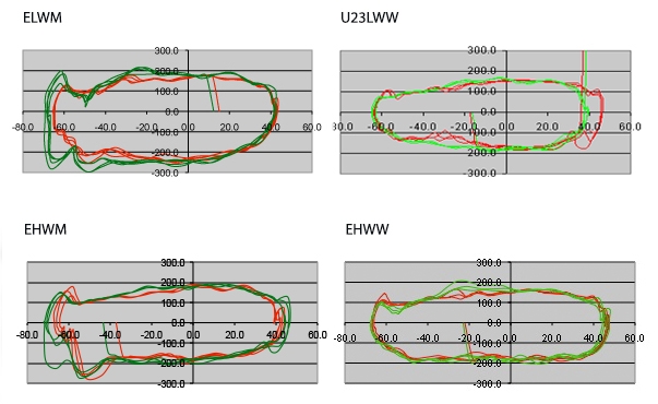
In the boat, the shape of the handle speed curve of the Recovery is almost a direct mirror of the Drive. This is evident by the handle speed curve of the U23 sculler (actually recorded when she was still an inexperienced junior) showing that the slow catch is mirroring a slow last part of the recovery. Ironically, at that stage of her development, her handle speed during the last part of the drive was the equal of the 3 Olympians, but her hands-away at the finish did not mirror and then her mid-recovery was rushed in comparison. This is a good example of the power of the handle speed curve for a kinematic analysis of the stroke cycle:
Using the ELM 1X handle speed curve as an example: At the furthest extension of approximately -65 degrees the angular acceleration of the handle goes from 0 to 200 radians (at least on the starboard {green} side). In almost no time the sculler matches the velocity of the boat relative to the water at about 5 m/s, its minimum. That is a graphical description of a very quick catch!
It shows what the scullers mass is doing because it is connected to the handle. Both the ELM and EHWM scullers show a very nice mirroring of the handle speed on the Recovery. When done correctly the complete handle speed curve shape resembles that of a snack food “little fish”!
What the recovery part of the curve shows is a measured speed of the hands as they come away, followed by the upper body swinging forward and than the rowers mass moving toward the Catch (left vertical side of the curve) at a velocity about equal to that of the drive, or about -200 radians at racing rates. The rowers mass then speeds up in conjunction with the square up just before the catch in an effort to continue the momentum and make de-acceleration of mass as short as possible.
Referring again to the Handle Speed Curves of the four examples of quite accomplished scullers. You will see the same characteristic curve at the catch with all of them where the handle speed is constrained by boat speed. The point that this makes is the futility and inefficiency of driving too hard with the legs initially. You must limit force until the boat progresses enough to have a favorable mechanical advantage with the leg angle. About 75% maximum pressure will be enough until the legs get to a biomechanically stronger position where you are able to drive down hard with the legs.
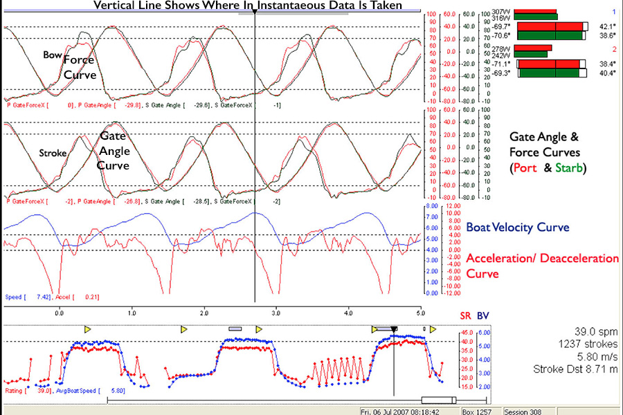
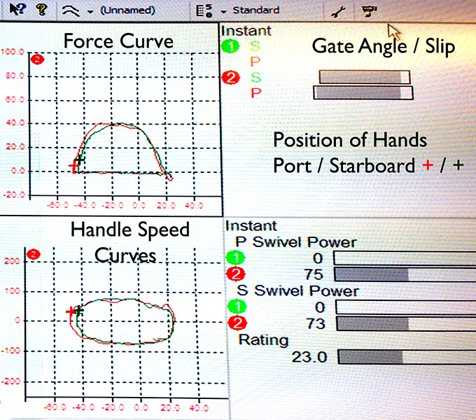
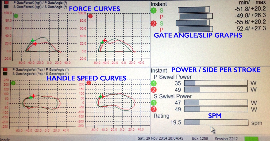
Instantaneous Tank Display:
Below are data curves from a display of an indoor tank equipped with a Force Measurement System. Shown are instantaneous Force Curves (Impulse Curves) and Handle Speed Curves with a red “+” indicating the position of the port hand and a green “+” for starboard hand, which also indicates the relative positioning of the hands on both sets of curves. Note the bar graphs on the right side are refreshed once per stroke. The curves are from two 16-year-old scullers (so we try not to be too judgmental). The more accomplished sculler is on the right (stroke) side. The less accomplished with regard to technique is on the left (bow).
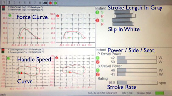
Reading the display going clockwise: Force curves are in the upper quadrant for both rowers with a red dot indicating port and the green dot starboard. The next quadrant is handle speed represented as a bar graph with the length of the bar representing stroke length and the relative starting point of each bar indicating the furthest catch angle for each side of each rower. Numerical catch angles are to the right of each bar. There is a threshold value of ten newtons that has to be exceeded before the bar is shaded and that visually represents the true catch. The length of shading represents total effective stroke length until the 10-newton threshold is crossed again. The goal here is to have no white showing at the start of the bar, indicating a quick catch. It is almost impossible to eliminate all the white at the end of the bar due to momentum. However, an excessive length of “white” indicates premature disengagement from the water (i.e., washing-out or pulling down into one’s lap).
The 3rd quadrant shows power per side for each sculler in watts and stroke rate. This is not absolute power but relative power because the mechanics of the tank are so much different from the boat that it is beyond the calibration range of the existing software.
The last quadrant shows the handle speed for each sculler. The shape and slope is similar to that seen in the boat, with the exception of immediately after the catch is more continuous mainly because the blade is being pulled through the water rather than being supported by the water and forced to match boat speed, as in the boat. The shape of the handle speed curve ends up looking like a “peanut”, curved downward at both ends with top and bottom mirroring one another.
The following video shows the same two young scullers using the tank and its Force Measurement System. You can hear me coaching them by questioning them: “When you accelerate your hands at the end of the stroke, what does that do to the shape of the (handle speed) curve?”. In this way, they learn by doing, assisted by real-time feedback. This is a much quicker, and more long-lasting coaching method, that works so much better than hoping that they will interpret your words correctly.
From experience, we have learned that if the rower is self-coaching in the tank, he or she can only effectively look at one quadrant at a time. By playing the video over-and-over you should see most of the following takeaways: The bow person (left side) has trouble with the side-to-side synergism as compared to the stroke person (right side). The slope of the curve at the catch is different between the bow and the stroke, and this is also reflected in the slip at the catch shown by the bar chart. What you don’t see or know is that the person in stroke seat has primarily sculled, whereas the bow person has primarily rowed sweep, The bow person is quite a bit taller in stature, but short on each end of the stroke. You can see that there is less handle speed acceleration during the stroke with the bow person than the stroke. There is a different hand speed away from the release of the recovery by the two athletes, which does not help synergism. The bow is being a bit excessive with hands out of the bow.
Problems like these can be easily seen and identified by the rowers in real time as well as by the coach. From our experience, identical problems occur on the water and in the tank. Once pointed out, the problems can usually be quickly fixed.
Also during the practice, a video can be made of the output data along with a video of what the problems look like from the stern or side-view and sent via cell phone immediately to the athlete. This is a very powerful tool. When environmental conditions of wind and weather, or school constraints impact training time, then real-time tank sessions are a much better use of coaching time then on-the-water sessions.
STEM Education Using Rowing Physics:
By now you should start to see the possibilities for rowing physics to be used as a “physics (and calculus) lab. All the basic physics mechanics properties have been touched on and shown to be hands-on ready for after school STEM education. This becomes particularly easy if you have access to a rowing tank equipped with a Force Measurement System. If you are lucky enough to have a rowing tank at your University, School or Club all that is needed is a Force Measurement System and a Physics/Math instructor and you will have sustainable income with both State and Federal funding available to help support your rowing program/STEM education program.
What has briefly been described above as an introduction to rowing physics could be easily expanded upon and made into a lesson plan by any secondary school or college physics instructor. Physics Mechanics based on rowing makes it easy to illustrate the very basic Newtonian Physics Principles. In like manner an introduction to the graphical representation of calculus, fluid dynamics, etc. could also be shown using a “hands-on” or heuristic approach using rowing mechanics as a lab model.
By: Jim Dreher, 06/27/17
One Response
Why I’m teaching kids science through the sport of rowing – Fairy Dell Farms
[…] basic principles of rowing appear quite simple, but in reality, rowing success is complex. Momentum is transferred to the water by pulling on the oar and pushing with the legs, which causes […]